Mirror Face

It seems that many friends are curious about the mirror face trick described in my paper. I am writing this technical report to describe it with more details.

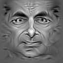
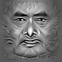
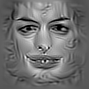
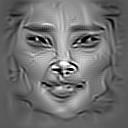
mirror

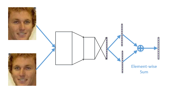
Mirror face is (one of) the most effective prior for face image analysis. It extracts features from the frontal face and mirror face simultaneously and merges the two features together as the final feature. A sample network is in FaceNormGithub/prototxt/example_of_mirror_face.prototxt.

Mirror face can be trained in an end-to-end manner. However, I find it has no help on training face verification models. It can improve the performance of face identification, but when I apply it on face verification, the accuracy even decreases:(

Here are the accuracies using Wen’s model with different feature merging strategy. We didn’t put these tables into our paper because we thought this was only a trick.

With my model:

And with Wu’s Light CNN B:

With my model:

It’s strange that with my C-contrastive loss, the performance of No PCA is better… Anyway, in Wu’s paper, he didn’t use PCA either. So there is nothing wrong with what I said in my paper: “I follow all the experiment settings of the original paper”.

To sum up, the mirror face trick is effective on most of the models (actually I never see cases that mirror face does not work). However, we are lacking the theoretical explanation for it. Now we can only explain it as model ensemble. Whether to use SUM or MAX, how to train it end-to-endly in face verification models, these are still open problems. Hope this report can inspire people to do further research.

In the last post, we have discussed how to normalize the gradients in the back propagate procedure. However, we left a problem about the stride parameter of the convolution layer and pooling layer. It is not an easy task so I tend to open a new post to discuss it.

In this article, we are looking at a convolution layer or pooling layer with $w\times w$ window and $s\times s$ stride. These two symbols are all the same in the following paragraphs. We will use FP to refer to the forward propagation and BP for backward propagation in short.

In the FP, we do not need to consider the stride parameter because every output pixel accumulates values from all input pixels of $w\times w$, no matter how much pixel strides are applied. However, in the BP procedure, each output pixel (input in FP) correspond to only a small subset of input pixels. Different from striding on the feature map during FP, we do stride on the kernel in BP. I have drawn a picture to illustrate this procedure.

As shown above, an input feature map is convolved by a $3\times 3$ filter with $2\times 2$ stride. We can see that different values on input map participate in the convolution with different times. 7, 9, 17, 19 are convolved only once, while 13 convolved $4$ times. Since BP is actually the inverse procedure of FP in convolution layer, if the kernel is all flat, the gradient at position 7 will be $4$ times smaller compared with the gradient at position 13.

There are two ways to normalize the output gradient. The first one is to scale the entire output gradient map. Please note that the Multiplication Count is constituted by some repeated cells, e.g. [4 2; 2 1] in the above figure. Then we can calculate the std of the output gradient:

$$Std[dx] = \sqrt{\frac{1}{4}(4^2 + 2^2+2^2+1^2)} = \frac{5}{2}.$$

Don’t forget that we have normalized the filter to have unit $\ell 2$ norm, i.e. we have already divided all the values in the filter by 3 in the above circumstance (channel = 1). So the final correction factor is $\frac{5}{6}$, we should divide the $\ell 2$ normalized gradients by this value. Other repeated cells used by a general network are recorded below.

Another way is to normalize the values in the filters. Since we can modify the filters arbitrarily, we may rescale each value in the filter matrix separately. The corners, which are shared by $4$ convolution windows as illustrated in the first figure, need to multiply a factor of $\frac{1}{4}$. Similarly, we should scale the edge values by $\frac{1}{2}$ and keep the central values unscaled because each of them only locates in one convolution window. The normalize factors of some small kernels are listed below.

Analysis of the stride parameter in the average pooling layer is similar. Since it can be seen as convolution layer with mean filters, the normalization strategy is the same with the first method we discussed above, scaling the whole gradient map by a specified value w.r.t the $w$ and $s$.

For max-pooling layers, things get different. There is a special case that the max value can be taken from the same position on the feature map but in different windows. This circumstance is very common because the image is usually continuous, a maximum value may be the only extreme value in a large region. Look at the two cases below. The max values are taken from different positions in the left case while the two windows share the same max value in the right case. The scale factor will be very different if we still use std as our measurement.

One solution is to use MAD(Mean Abs Deviation) instead of standard deviation as the measurement for the scale. The formulation of MAD is

$$ MAD(x) = \frac{1}{N}\sum_i^N{|x_i-E[x]|}.$$

To be compatible with MAD, we need to change our hypothesis introduced in the last two posts from Gaussian distribution to Laplacian distribution. This will be a huge work and I will write the derivation of the formulations in the next post.

1.Introduction

In the last post, we discussed how to make all neurons of a neural network to have normal Gaussian distribution. However, as the Conclusion section claimed, we haven’t considered the back-propagation procedure. In fact, when we talk about the gradient vanishing or exploding problem, we usually refer to the gradients flow in the back-propagation procedure. Since this, the correct way seems to be normalizing the backward gradients of neurons, instead of the forward values.

In this post, we will discuss how to normalize all the gradients using a similar philosophy with the last post: for a given gradient \(dy\sim N(0, I)\), normalizing the layer to make sure that \(dx\) is expected to have zero mean and one standard deviation.

2. Parametric Layer

Consider the back-propagate fomulation of Convolution and InnerProdcut layer,

\[dx = W dy,\]

we will get a similar strategy of normalizing each row of \(W\) to be on a \(\ell 2\) unit ball. Please note that here we normalize through the fan-out dimension of \(W\), not the fan-in dimension in the forward propagation.

3. Activation Layers

One problem that can’t be avoided when calculating the formulations of activations is that we should not only assume the distribution of the gradients, but also the forward input of the activation because the gradients of activations are usually dependent on the inputs. Here we assume that both the input \(x\) and the gradient \(dy\) follow the normal Gaussian distribution \(N(0, I)\), and they are independent with each other.

1) ReLU

The forward formulation of ReLU is,

\[y = max(0, x).\]

Its backward gradients can be easily obtained:

\[dx_i = dy_i * \left\{ \begin{array}{rcl} 1 & & {x_i > 0}\\ 0 & & {x_i \leq 0}. \end{array} \right.\]

When \(x\sim N(0, I)\), the gradient of the ReLU layer can be seen as a Bernoulli distribution with probability of 0.5, so the backward mean and standard deviation formulas are similar with those of Dropout layer,

\[E[dx] = 0,\]

\[\sigma[dx]=\sqrt{\frac{1}{2}}.\]

Here the question comes, now we have two different standard deviations, one for forward values and one for backward gradients, which one should be used to normalize the ReLU layer? My tendency is to use the \(\sigma\) calculated by the backward gradients, because backward \(\sigma\) is the real murderer of gradient vanishing. Moreover, since the bias term is not involved in the backward propagation, it is a good manner to substract the mean \(\sqrt{\frac{1}{2\pi}}\) after ReLU activation to ensure zero mean.

2) Sigmoid

The backward gradient of Sigmoid activation is,

\[ dx = y \cdot (1-y).\]

This time, I won’t attempt to calculate the close formulations of mean and std, it is really a tough work. I tend to directly use simulating to get the results.

1
2
3
4
5

x = randn(100000,1);
y = 1 ./ (1 + exp(-x));
dy = randn(100000,1);
dx = dy .* y .* (1-y);
disp([mean(dx) std(dx)]);

We can get \(E[dx] = 0\) and \(\sigma[dx]=0.2123\). The same with ReLU, we should still minus the \(E[y]=0.5\) after Sigmoid activation and use the \(\sigma\) calculated by backward gradients, 0.2123.

4. Pooling Layer

The standard deviation of \(3\times3\) average pooling can be simulated by,

1
2

dx = [randn(100000,9) / 9];
disp(std(dx(:)));

It is \(\frac{1}{9}\), and we can infer that the \(\sigma\) for \(2\times2\) average pooling is \(\frac{1}{4}\).

For max pooling, we only pass the gradient to one of the neurons in the pooling window, so we have,

1
2
3

dy = randn(100000,1);
dx = [dy zeros(100000,8)];
disp(std(dx(:)));

Running the script and we can get \(\sigma\) for \(3\times3\) is \(\frac{1}{3}\) and \(\sigma\) for \(2\times2\) is \(\frac{1}{2}\).

5. Dropout Layer

The backward formula for Dropout layer is almost the same with the forward one, we should still divide the preserved values by \(\sqrt{q}\) to achieve 1 std for both forward and backward procedure.

6. Conclusion

In this post, we have discussed the normalization strategy that serves the gradient flow of the backward propagation. The mean and std values of forward and backward data flows are listed here:

However, here comes another problem that when we are using the std of backward gradients, the forward value scale would not be controlled well. Inhomogeneous(非齐次) activations, such as sigmoid and tanh, are not suitable for this method because their domain may not cover a sufficient non-linear part of the activation.

So maybe a good choice is to use a separate scaling method for forward and backward propagation? This idea conflicts with the back-propagation algorithm, so we should still carefully examine it through experiment.

This article is a note on 《Normalization Propagation: A Parametric Technique for Removing Internal Covariate Shift in Deep Networks》.

1. Introduction

If you are doing research in Deep Learning, you must know the Batch Normalization[3] technique, which is a powerful tool to avoid internal covariate shift and gradient vanishing. However, batch normalization only normalizes the parametric layers such as convolution layer and innerproduct layer, leaving the chief murderer of gradient vanishing, the activation layers, apart. Another disadvantage of BN is that it is data-dependent. The network may be unstable when the training samples are in high diversity, or training with small batch size or our objective is a continuous function such as regression.

In [1], the authors proposed a new standard that if we feed a uniform Gaussian distributed data into a network, all the intermediate output should also be uniform Gaussian distribute, or at least expected to have zero mean and one standard deviation. In this manner, the data flow of the whole network will be very stable, no numerical vanishment or explosion. Since this method is data-independent, it is suitable for regression tasks or training with the batch size of 1.

2. Parametric Layers

For parametric layers, such as convolution layer and innerproduct layer, they have a mathematic expression as,

\[y = W^Tx.\]

Here we express the convolution layer in an inner-product way, i.e. using im2col operator to convert the feature map into a wide matrix \(x\).

Now we assume that \(x\sim N(0, I)\), our objective is to let each element in \(y\) also follows a uniform Gaussian distribution, or at least each value is expected to have zero mean and variance is 1. We can easily find that \(E[y]=0\) and

\[Cov[y] = E[yy^T] = E[W^Txx^TW] = W^TE[xx^T]W = W^TW.\]

Let \(W_i\) to be the ith row of \(W\), then \(\Vert W_i\Vert _2\) must equals to 1 to satisfy our target. So a good way to control the variance of each parametric layers’ output is to force each row of the weight matrix to be on a \(\ell 2\) unit ball.

To achieve this, we may scale the weight matrix during feed forward,

\[\tilde{W_i} = \frac{W_i}{\Vert W_i \Vert _2},\]

and in back propagation a partial derivative is used:

\[\frac{\partial \ell}{\partial W_i} = \frac{\frac{\partial \ell}{\partial \tilde{W_i}} - \tilde{W_i}\sum_j{\frac{\partial \ell}{\partial \tilde{W_{ij}}}\tilde{W_{ij}}}} {\Vert W_i \Vert _2}.\]

Or, we can directly use the standard back propagation to update \(W\) and force to normalize it after each iteration. Which one is better still need examination by experiment.

3. Activation Layers

Similar with the parametric layers, we also require the post-activation values to have zero mean and 1 standard deviation.

1) ReLU

We all know that the formula of ReLU is,

\[y = max(x, 0).\]

Assuming \(x\sim N(0,I)\), we can obtain,

\[E[y] = \int_{0}^{+\infty}x\frac{1}{\sqrt{2\pi}}e^{-\frac{x^2}{2}}dx= \frac{1}{\sqrt{2\pi}}\int_{0}^{+\infty}e^{-\frac{x^2}{2}}d\frac{x^2}{2}.\]

It can be easily got, \(E[y] = \sqrt{\frac{1}{2\pi}}\). Then

\[E[y^2] = \int_{0}^{+\infty}x^2\frac{1}{\sqrt{2\pi}}e^{-\frac{x^2}{2}}dx= \frac{1}{2}\int_{-\infty}^{+\infty}x^2\frac{1}{\sqrt{2\pi}}e^{-\frac{x^2}{2}}dx = \frac{1}{2},\]

\[Var[y] = E[y^2] - E[y]^2=\frac{1}{2} - \frac{1}{2\pi}.\]

Thus, we should normalize the post-activation of ReLU by substracting \(\sqrt{\frac{1}{2\pi}}\) and dividing \(\sqrt{\frac{1}{2} - \frac{1}{2\pi}}\).

2) Sigmoid

The formula of Sigmoid activation is,

\[y = \frac{1}{1+e^{-x}},\]

\[E[y] = \int_{-\infty}^{+\infty}\frac{1}{1+e^{-x}}\frac{1}{\sqrt{2\pi}}e^{-\frac{x^2}{2}}dx \\ =\int_{-\infty}^{+\infty}(\frac{1}{1+e^{-x}}-\frac{1}{2}+\frac{1}{2})\frac{1}{\sqrt{2\pi}}e^{-\frac{x^2}{2}}dx\\ =\int_{-\infty}^{+\infty}(\frac{1}{1+e^{-x}}-\frac{1}{2})\frac{1}{\sqrt{2\pi}}e^{-\frac{x^2}{2}}dx +\frac{1}{2}\\ =0+\frac{1}{2}=\frac{1}{2},\]

\[E[y^2] = \int_{-\infty}^{+\infty}(\frac{1}{1+e^{-x}})^2\frac{1}{\sqrt{2\pi}}e^{-\frac{x^2}{2}}dx.\]

OK, I don’t think we can get a close form of the integral part of \(E[y^2]\). Please note that we are not using the exact form of the equation. What we need is only an empirical value, so we can get the numbers by simulating. With a huge amount of random values, say 100,000, we can get relatively accurate means and standard derivations. By running the script in Matlab,

1
2
3

x = randn(100000,1);
y = 1 ./ (1 + exp(-x));
disp([mean(y) std(y)]);

we can get Sigmoid’s standard deviation: 0.2083. This value can be directly written into the program to let the post-sigmoid value have 1 standard deviation.

4. Pooling Layer

There are two types of pooling layer, average-pooling and max-pooling. For the average-pooling layer, it is easy to infer that \(E[y] = 0\) and \(Std[y] = \frac{1}{\sqrt{n}} = \frac{1}{s}\), where \(n\) is the number of neurons in a pooling window or \(s\) is the side length of a square pooling window.

For the max-pooling layer, there is no close form expressions either. We still use the simulated values generated by,

1
2
3

x = randn(10000000, 9);
y = max(x, [], 2);
disp([mean(y) std(y)]);

The mean value of a \(3\times3\) max-pooling is 1.4850 and the standard deviation is 0.5978. For \(2\times2\) max-pooling, mean is 1.0291 and standard deviation is 0.7010.

5. Dropout Layer

Dropout is also a widely used layer in CNN. Although it is claimed to be useless in the NormProp paper, we still would like to record the formulations here. Dropout randomly erases values with a probability of \(1-p\). Now we write it into a mathematic form,

\[y = x \odot r,\]

where \(r\sim Bernoulli(p)\). Thus,

\[E[y] = \sum_{i=0,1}\int_{-\infty}^{+\infty}{xr_ip_i\frac{1}{\sqrt{2\pi}}e^{-\frac{x^2}{2}}}dx\\ =0 * \int_{-\infty}^{+\infty}{x(1-p)\frac{1}{\sqrt{2\pi}}e^{-\frac{x^2}{2}}}dx + 1 * \int_{-\infty}^{+\infty}{xp\frac{1}{\sqrt{2\pi}}e^{-\frac{x^2}{2}}}dx\\ =0\]

\[E[y^2] = \sum_{i=0,1}\int_{-\infty}^{+\infty}{(xr_i)^2p_i\frac{1}{\sqrt{2\pi}}e^{-\frac{x^2}{2}}}dx\\ =0+\int_{-\infty}^{+\infty}{x^2p\frac{1}{\sqrt{2\pi}}e^{-\frac{x^2}{2}}}dx\\ =p\]

\[Std[y] = \sqrt{E[y^2]-E[y]^2}=\sqrt{p}\]

Interestingly, this result is different from what we usually do. We usually preserve values with a ratio of \(p\) and divide the preserved values by \(p\), too. Now as we calculated, to achieve 1 s.t.d., we should divide the preserved values by \(\sqrt{p}\). This result should be carefully examined by experiment in the future.

6. Conclusion

In this report, we followed the methodology of [1] to infer the formulation for normalizing all popular layers of a modern CNN. We believe that normalizing every layer with mean substracted and s.t.d. divided will become a standard in the near future. Now we should start to modify our present layers with the new normalization method, and when we are creating new layers, we should keep in mind to normalize it with the method introduced above.

The shortage of this report is that we haven’t considered the back-propagation procedure. In paper [1][4], they claim that by normalizing the singular values of Jacobian matrix to 1 will lead to faster convergence and more numerically stable. I will study them and explore how to integrate the Jacobian normalization into the present normalization method.

Reference

[1] Devansh Arpit, Yingbo Zhou, Bhargava U. Kota, Venu Govindaraju, Normalization Propagation: A Parametric Technique for Removing Internal Covariate Shift in Deep Networks. http://arxiv.org/abs/1603.01431

[2] Tim Salimans, Diederik P. Kingma, Weight Normalization: A Simple Reparameterization to Accelerate Training of Deep Neural Networks. http://arxiv.org/abs/1602.07868

[3] Sergey Ioffe, Christian Szegedy, Batch Normalization: Accelerating Deep Network Training by Reducing Internal Covariate Shift. http://arxiv.org/abs/1502.03167

[4] Andrew M. Saxe, James L. McClelland, Surya Ganguli, Exact solutions to the nonlinear dynamics of learning in deep linear neural networks. http://arxiv.org/abs/1312.6120

Appendices

A. The formula fault of [1]

In [1], they present a bound describing the error of using diagnose matrix to approximate a covariance matrix. However, the bound is wrong. They mistake the \(\Vert W_i\Vert_2^4\) by \(\Vert W_i\Vert_2^2\) in the last line of equation 18. Then the equation 3 and 19 become to:

\[\Vert \Sigma - diag(\alpha) \Vert_F^2\le \sigma^4 \sum_{i,j=1;i\ne j}^m{m(m-1)\mu^2 \Vert W_i \Vert_2^2 \Vert W_j \Vert_2^2}\]

As we can see, there is no \(1- \Vert W_i \Vert_2^2\) at all, so there is no reason to explain why we should normalize \(\Vert W_i \Vert_2^2=1\).

However, they still get the correct conclusion that we should normalize the weight matrix by the \(\ell 2\) norm of rows. But the theoretical analysis of the bound is wrong. In fact, the reason why we should normalize the weight matrix is very simple as we wrote above.

1. Introduction

Machine Learning researchers may split the learned model into two categories, generative model and discriminative model. Convolutional Neural Network is usually seen as a powerful discriminative model. We used to think that the discriminative model has no ability to generate the whole image, just as we human beings, we cannot draw a vivid picture without professional training.

Now we all know that the CNN based system has surpassed human beings in the ability to recognize people. So do the discriminative CNNs have a better ability to draw portraits, even trained with only discriminative signals? This post will tell you the answer.

Firstly, we need to find a CNN model which is close to the human beings in recognizing people. Thanks Wu Xiang. He has provided a model with 98.13% verification rate on LFW, while human beings’ average rate is about 99%. We will use the model he provided for the following experiments.

2. Method

If you are interested in Deep Learning, you must know the Inceptionism, which have raised a huge wave of using Neural Networks for art making. Here we will use a similar tool, reversing the neural network. Different from what we usually do, giving an image to a CNN model and it tells us this is Susan or Lucy, now we will tell the neural network from the tail of CNN that we need Susan’s image. Then by back-propagation, we will finally get an image from the input side of the CNN model.

3. Result

Wu Xiang’s model is trained with CASIA-WebFace dataset, which is very huge, containing about 490,000 face images of 10,575 movie stars. Now, let’s see choose some movie stars and see what they look like in computer’s brain:

Bruce Lee	Mr. Bean

Yun-Fat Chow	Anne Hathaway

Bingbing Li	Bingbing Fan

LoL, are these portraits somewhat look like them in the real world? We can see that the CNN have indeed memorized some features of the training samples, not as the all along prejudice that discriminative model cannot do generating tasks. They can, and do well!

PS: I can’t wait to show the images generated by a pornography detection system. If you have trained one, please contact me!

PS2: The codes are on my Github. The face verification model can be found in Wu Xiang’s Github.

PS3: A friend of mine gave me a pedestrian detection model. Here is its visualization. I believe you can find a “fat person” in it, LOL.

pedestrian

This article is from a failed work. If you can read Mandarine, please see this blog for details. I have underestimated the effect of scale & shift in Batch Normalization. They are very important!

However, I don’t want this work to be thrown into dust basket. I still think that we can get some interesting and direct feelings from the generated images.

Brief Algorithm Description

Firstly we take a two channel “slope” image as input.

first channel	second channel

Then we use a randomly initialized (convolutional) neural network to wrap the slope input to some more complex shapes. Note that a neural network is continuous function w.r.t. the input, the output will also be a continuous but more complex image.

In order to control the range of each layers’ output, we add batch normalization after every convolutional layer as introduced in the original paper. BTW, since we have only one input image, the name “batch normalization” is better to be changed to “spatial normalization”. Without the spatial normalization, the range of the output will get exponential increase or decrease with the depth, which is not what we want.

Now we can see how complex the neural network could be. Firstly, with a single layer, 100 hidden channels.

ReLU activation	Sigmoid activation

How about 10 layers with 10 hidden channels respectively?

ReLU activation	Sigmoid activation

Much more complex, right? Please note that they all have about 100 parameters, but with deeper structure, we produce images with a huge leap in complexity.

We can also apply other structures on the input, such as NIN, VGG, Inception etc, and see what’s the difference of them.

The codes are all on my github, you may try them by yourself!

Recently, I noticed that there were similar works long ago. This algorithm is called Compositional pattern-producing network and some other posts also generates beautiful images, such as http://blog.otoro.net/2016/03/25/generating-abstract-patterns-with-tensorflow/ and http://zhouchang.info/blog/2016-02-02/simple-cppn.html .