In the last post, we have discussed how to normalize the gradients in the back propagate procedure. However, we left a problem about the stride parameter of the convolution layer and pooling layer. It is not an easy task so I tend to open a new post to discuss it.
In this article, we are looking at a convolution layer or pooling layer with $w\times w$ window and $s\times s$ stride. These two symbols are all the same in the following paragraphs. We will use FP to refer to the forward propagation and BP for backward propagation in short.
In the FP, we do not need to consider the stride parameter because every output pixel accumulates values from all input pixels of $w\times w$, no matter how much pixel strides are applied. However, in the BP procedure, each output pixel (input in FP) correspond to only a small subset of input pixels. Different from striding on the feature map during FP, we do stride on the kernel in BP. I have drawn a picture to illustrate this procedure.
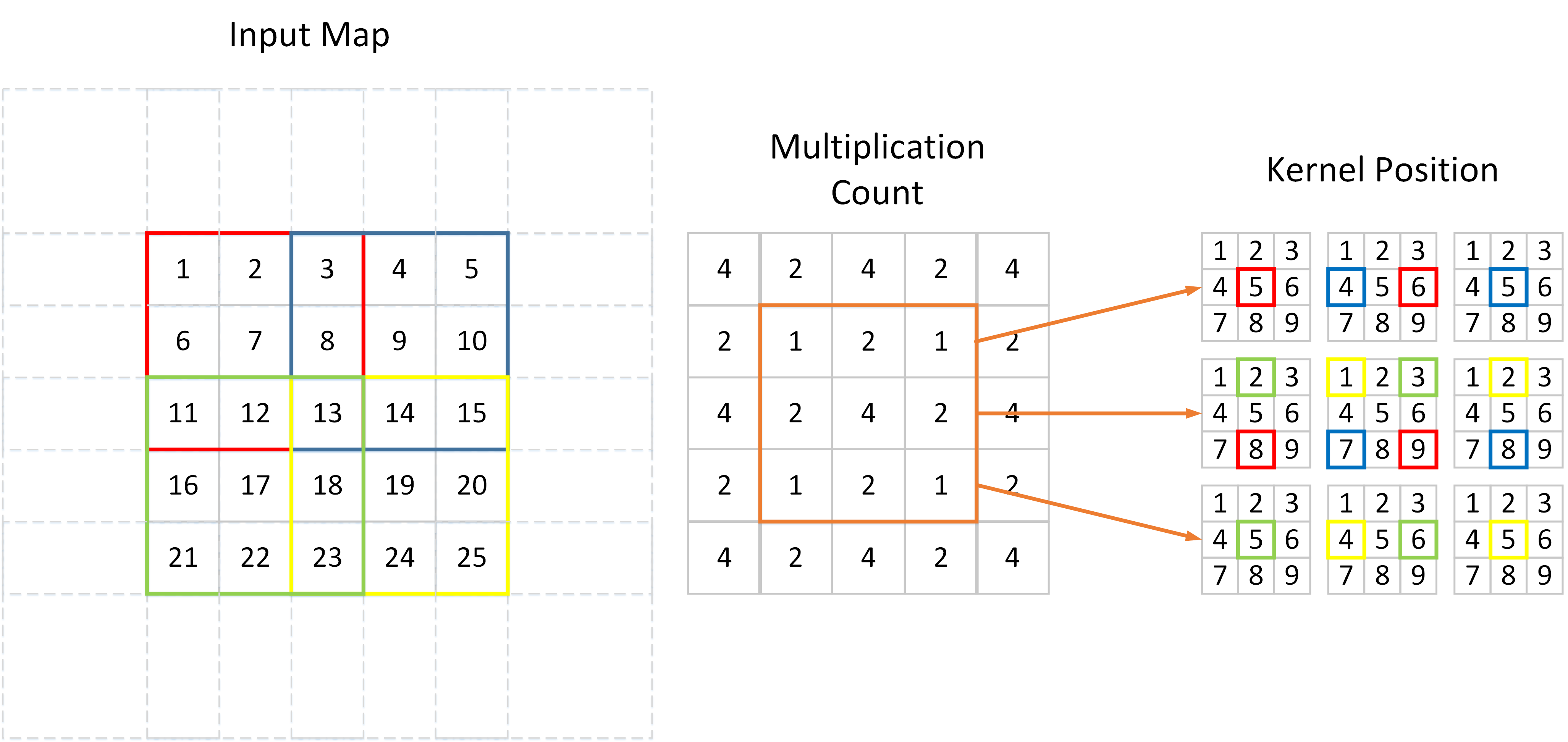
As shown above, an input feature map is convolved by a $3\times 3$ filter with $2\times 2$ stride. We can see that different values on input map participate in the convolution with different times. 7, 9, 17, 19 are convolved only once, while 13 convolved $4$ times. Since BP is actually the inverse procedure of FP in convolution layer, if the kernel is all flat, the gradient at position 7 will be $4$ times smaller compared with the gradient at position 13.
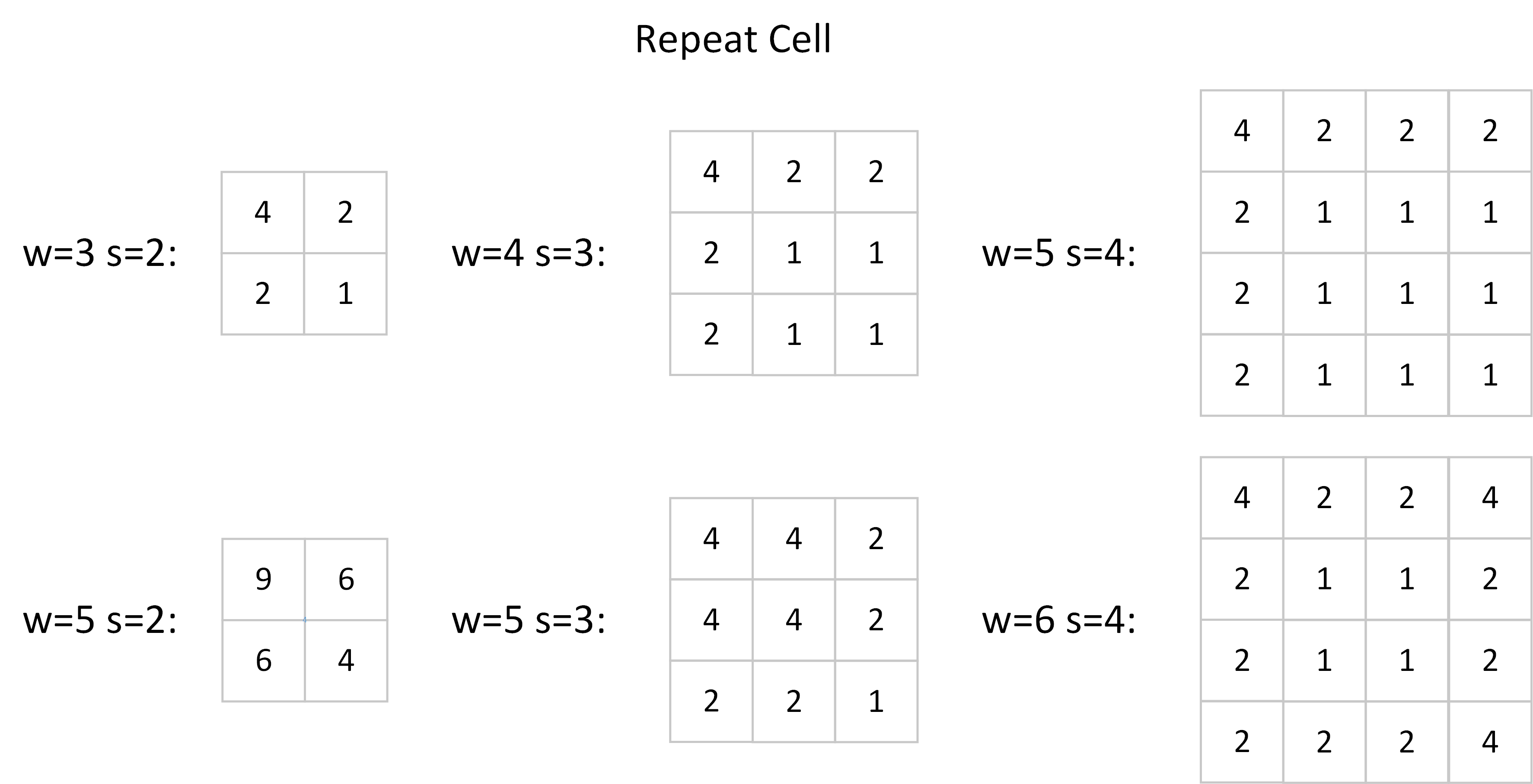
There are two ways to normalize the output gradient. The first one is to scale the entire output gradient map. Please note that the Multiplication Count is constituted by some repeated cells, e.g. [4 2; 2 1] in the above figure. Then we can calculate the std of the output gradient:
$$Std[dx] = \sqrt{\frac{1}{4}(4^2 + 2^2+2^2+1^2)} = \frac{5}{2}.$$
Don’t forget that we have normalized the filter to have unit $\ell 2$ norm, i.e. we have already divided all the values in the filter by 3 in the above circumstance (channel = 1). So the final correction factor is $\frac{5}{6}$, we should divide the $\ell 2$ normalized gradients by this value. Other repeated cells used by a general network are recorded below.
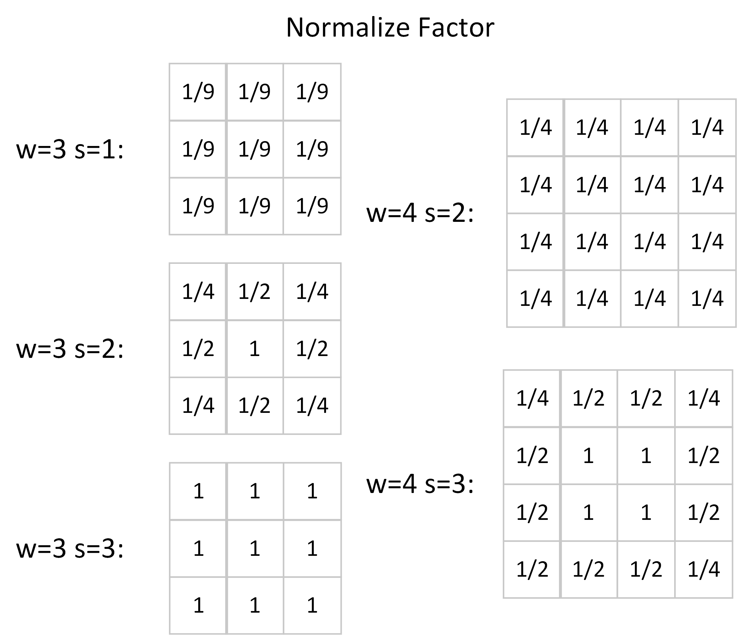
Another way is to normalize the values in the filters. Since we can modify the filters arbitrarily, we may rescale each value in the filter matrix separately. The corners, which are shared by $4$ convolution windows as illustrated in the first figure, need to multiply a factor of $\frac{1}{4}$. Similarly, we should scale the edge values by $\frac{1}{2}$ and keep the central values unscaled because each of them only locates in one convolution window. The normalize factors of some small kernels are listed below.
Analysis of the stride parameter in the average pooling layer is similar. Since it can be seen as convolution layer with mean filters, the normalization strategy is the same with the first method we discussed above, scaling the whole gradient map by a specified value w.r.t the $w$ and $s$.
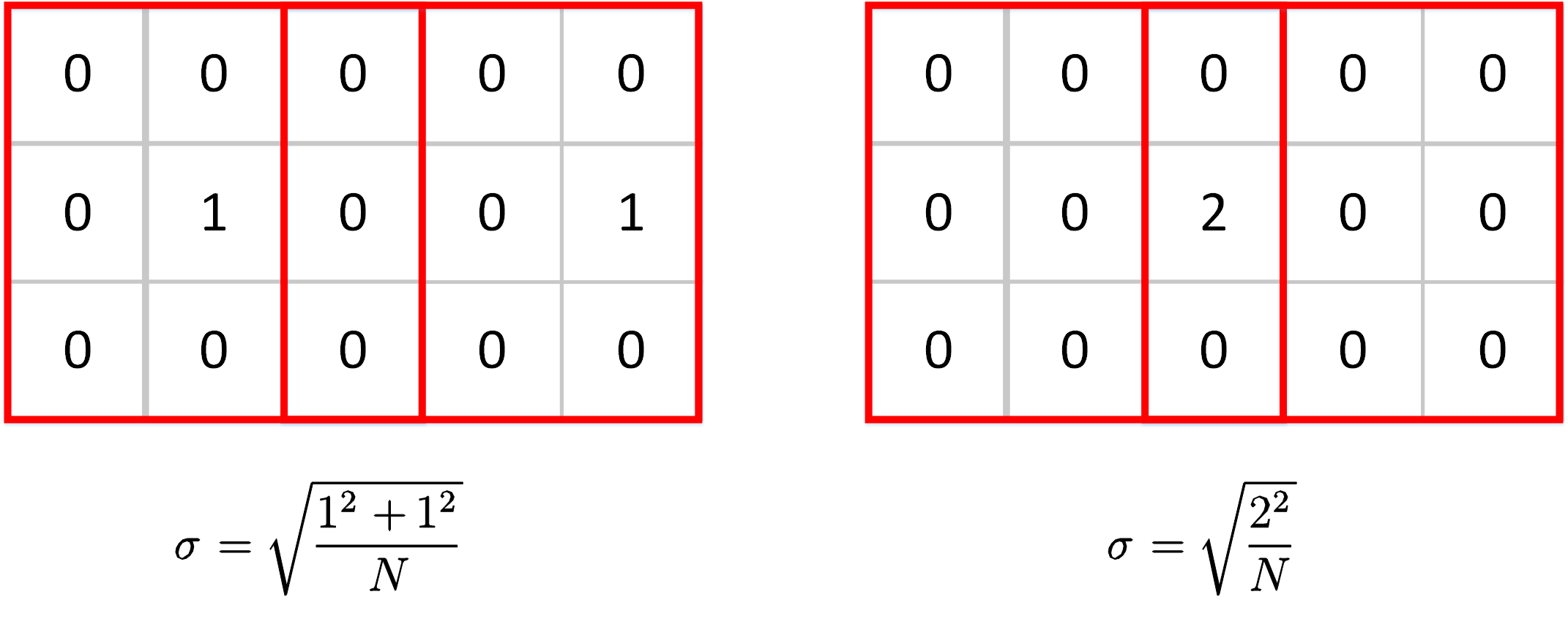
For max-pooling layers, things get different. There is a special case that the max value can be taken from the same position on the feature map but in different windows. This circumstance is very common because the image is usually continuous, a maximum value may be the only extreme value in a large region. Look at the two cases below. The max values are taken from different positions in the left case while the two windows share the same max value in the right case. The scale factor will be very different if we still use std as our measurement.
One solution is to use MAD(Mean Abs Deviation) instead of standard deviation as the measurement for the scale. The formulation of MAD is
$$ MAD(x) = \frac{1}{N}\sum_i^N{|x_i-E[x]|}.$$
To be compatible with MAD, we need to change our hypothesis introduced in the last two posts from Gaussian distribution to Laplacian distribution. This will be a huge work and I will write the derivation of the formulations in the next post.